Control series — a sketchbook
In one sentence
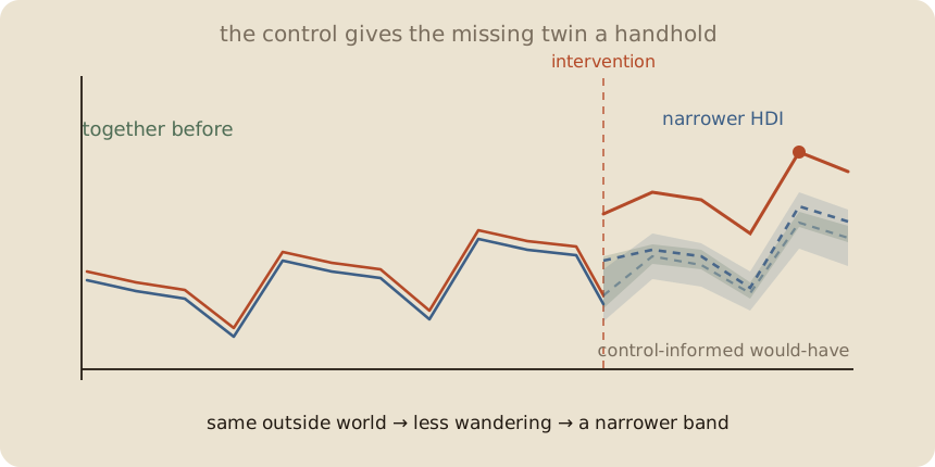
An unaffected, related series helps BSTS predict the missing would-have; because it explains more of the outside world, the counterfactual can have a narrower HDI.
Read 02 causal impact first. That note made the missing twin: what the treated series would have done without the campaign. This is the next question: what helps us draw that twin?
Page 1 — One series leaves a lot unknown
Class A gets extra office hours in week 17. After that, we see A. We do not see the other A — the A that never got the campaign.
Without another clue, many futures could fit the past:
- the class was going to climb
- a break was coming
- the whole school had a good week
- the campaign added something
The would-have is not a fact waiting behind the curtain. It is a prediction. A prediction has uncertainty.
Page 2 — A control is another window
Class B follows the same term. It gets the same breaks and outside shocks. It does not get the office-hours campaign.
B is a control series. It is not required to stay flat. In fact, a useful control moves when the outside world moves.
Before week 17, A and B should move together. If B rises and A usually rises too, later B helps us guess the A we would have had.
The control does not reveal the answer. It gives the prediction another handhold.
Page 3 — A band, not a line
BSTS — Bayesian structural time series — does not promise one perfect dashed line. It keeps a pile of plausible lines.
People often draw that pile as a credible band around the would-have. A 95% HDI is the shortest interval containing the densest 95% of the posterior draws in this small picture.
The band is uncertainty about the missing world. It is not uncertainty about whether the observed A value exists.
With A alone, the band may be wide. A good control explains some of the movement, so the band may become narrower.
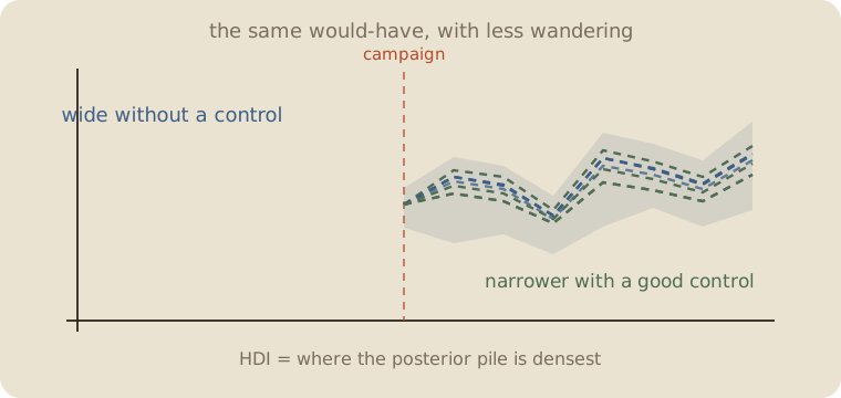
Narrower is not automatically better. A control that was also affected, or that never moved with A, adds confidence theater, not information.
Page 4 — Why the control can narrow the HDI
The model learns the old relationship between A and B before the campaign.
If B is high in a later week, the model has a better idea where A would probably be. Less of the prediction is left to the trend, the season, and the model’s vague prior.
In a Bayesian sketch:
- Start with possible relationships between A and B.
- Look at the pre-campaign weeks.
- Keep relationships that fit those weeks.
- Carry each surviving relationship through the later B values.
- The pile of resulting A paths is the counterfactual posterior.
The control can make that pile less spread out. That is the HDI getting narrower.
The condition is the important part:
not affected by the intervention, but affected by the same outside world.
Page 5 — One small number
In the toy class data, the pre-period relationship is strong: correlation 0.98.
At week 21, a simple model with trend and season alone gives a 95% posterior predictive interval of 6.01 to 7.51. Width: 1.49.
Give the model the good control series. The interval becomes 5.81 to 7.07. Width: 1.26.
The control shaved off some uncertainty. It did not prove the campaign worked. The observed A is 7.47; the causal question is still whether the control was truly unaffected and the pre-period relationship deserved trust.
Page 6 — Mini recipe
- Name the treated series and the intervention date.
- Find a series the intervention did not touch.
- Check that the two series moved together before the intervention.
- Fit the control, trend, and season on the pre-period only.
- Draw many possible would-haves. Keep the middle story and its HDI.
- Compare actual with the counterfactual band after the start.
- If the control was affected too, throw the shortcut away.
If you keep only one thing:
A good control does not remove uncertainty. It gives uncertainty less room to wander.
Page 7 — A control narrows the band, in numpy
This is a small Bayesian linear model, not a full BSTS package. It uses the same office-hours story to show the one lever that matters here: a related control can make the posterior predictive HDI narrower.
import numpy as np

rng = np.random.default_rng(7)
n = 24
t = np.arange(n, dtype=float)
season = np.array([0.8, 0.4, 0.1, -1.4] * 6)
control = 2.8 + 0.09 * t + 0.8 * season + rng.normal(0, 0.18, n)
y0 = 1.2 + 1.0 * control + 0.2 * season + rng.normal(0, 0.22, n)
start = 16
y = y0.copy()
y[start:] += 0.90

sigma = 0.28
prior_sd = 10.0

def posterior(X, y):
    precision = X.T @ X / sigma**2 + np.eye(X.shape[1]) / prior_sd**2
    covariance = np.linalg.inv(precision)
    mean = covariance @ (X.T @ y / sigma**2)
    return mean, covariance

def hdi(draws, mass=0.95):
    draws = np.sort(draws)
    width = int(np.floor(mass * len(draws)))
    spans = draws[width:] - draws[:-width]
    i = np.argmin(spans)
    return draws[i], draws[i + width]

def predictive_hdi(X, y, x_new):
    mean, covariance = posterior(X, y)
    beta = rng.multivariate_normal(mean, covariance, 12000)
    draws = rng.normal(beta @ x_new, sigma)
    lo, hi = hdi(draws)
    return draws.mean(), lo, hi

season_rows = np.eye(4)[np.arange(n) % 4][:, :3]
X_plain = np.column_stack([np.ones(n), t, season_rows])
X_control = np.column_stack([np.ones(n), control])
x_plain = np.array([1, 20, *season_rows[20]])
x_control = np.array([1, control[20]])

plain = predictive_hdi(X_plain[:start], y[:start], x_plain)
with_control = predictive_hdi(X_control[:start], y[:start], x_control)

print("pre-period correlation", round(np.corrcoef(control[:start], y[:start])[0, 1], 2))
print("week 21 actual A", round(y[20], 2))
print("without control mean / 95% HDI", round(plain[0], 2),
      np.round(plain[1:], 2))
print("with control mean / 95% HDI   ", round(with_control[0], 2),
      np.round(with_control[1:], 2))
print("HDI widths", round(plain[2] - plain[1], 2),
      "→", round(with_control[2] - with_control[1], 2))
pre-period correlation 0.98
week 21 actual A 7.47
without control mean / 95% HDI 6.74 [6.01 7.51]
with control mean / 95% HDI 6.42 [5.81 7.07]
HDI widths 1.49 → 1.26
The control makes this toy band 0.23 hours narrower. That is a prediction improvement, not a causal verdict. BSTS adds more structural pieces and a more careful posterior; the logic stays the same.
Last page — cheat sheet
| word | meaning |
|---|---|
| control series | a related series the intervention did not affect |
| pre-period | time before the intervention; where the relationship is learned |
| counterfactual | the treated series’ would-have without the intervention |
| HDI | shortest interval containing the densest posterior mass |
| BSTS | Bayesian structural time series: controls + trend / season + uncertainty |
Use / skip
Reach for it when
- you have a plausible unaffected series
- it moved with the treated series before the intervention
- you want uncertainty around the would-have, not one confident line
Skip it when
- the control received the intervention too
- the control and treated series never moved together
- you only need a next-week forecast (01 lag trend season)
Pays you: a more informed counterfactual and, when the control is good, a narrower HDI.
Costs you: a control is an assumption. A narrower band can still be precisely wrong if the control was contaminated or the relationship broke.
*A control carries some of the outside world. BSTS turns that clue into a distribution of would-haves.